The Power in the Power Function
So all the power in power functions comes from that little "b". Lets explore what values b can take on and how it changes the shape of the function. To do that, lets again consider a simplified version of our equation (this time, "a" is equal to 1):
Metabolic Rate = 1*Sizeb = Sizeb
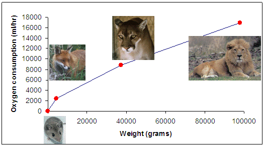
We already know what the relationship looks like for our four mammals:

To do that, we are going to explore the shape of the power function for three different ranges of "b": when b is greater than 1, between 0 and 1, and less than zero. We are going to show you how the graph of the function looks, determine what it suggests about the relationship of size with metabolic rate. We'll use the graph above as a guide, but while we do that, lets keep in mind that the above graph only represents four mammals - and may not be typical - so while we explore the behavior of the function as we change the value of "b", lets keep an eye out for which values of "b" seem to be biologically plausible for the metabolic rate - size relationship.
Below, we show for each of our three ranges of "b", a verbal description of what it means for "b" to be within each range, what the function looks like, describe what it means biologically, then decide if it is plausible to believe that "b" would take on that value. Remember, since "b" is an exponent (Metabolic Rate = Sizeb), we are really exploring the behavior of exponents!
|
b > 1
|
0 < b ≤ 1
|
b ≤ 0
|
|
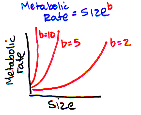
What happens when you raise a number to a value
greater than 1? What happens if you square a number, or raise it to the power of
5 or 10? The resulting value gets bigger and bigger at a faster and faster rate.
|
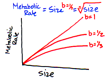
When you raise a number to the power of 1,
then its equal to itself (and therefore is linear). When its less than 1 you
are effectively taking a "root" of the number (so X1/2 is the
same as the square root of X).
|
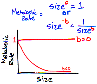
When you raise a number to the power of zero, the
resulting number = 1. When you raise a number to a negative exponent, its equivalent
to that same number raised in the denominator (so, X- b is equivalent to 1/ Xb).
|
|
|
|
|
|
So, if "b" is greater than 1, that means that as
size increased, metabolic rate would also increase, but faster and faster.
For example, if you compared the metabolic rates of an Indian elephant to an African
elephant (who is just a little bigger), that you would see a massive increase
in metabolic rate. That doesn't make any sense!
|
When b is equal to 1, then size increases linearly with metabolic
rate. When b is less than 1, it means that as size increases, metabolic rate also
increases, but it increases more and more slowly as organisms get bigger and bigger.
Hey! That looks looks like the relationship for our mammal graph (see above).
|
Neither of these make any sense at all! If
"b" is equal to 0, then metabolic rate is always 1. Clearly preposterous!
If "b" is negative, then as organisms get larger, their metabolic rate
gets closer and closer (but never reaches) 0. Another ridiculous pattern!
|
|
VERDICT: NO WAY!
|
VERDICT: This makes sense biologically!
|
VERDICT: NO WAY!
|
Oh - a bit of vocabulary. When b = 1, then the relationship remains consistent over all size classes. This is called an
"isometric" relationship. If the relationship changes across size classes (so b ≠ 1), it is called
"allometric". That's why scaling studies are often referred to as the field of "allometry". Although
(for whatever reason), when people refer to the field of allometry, they are usually referring to studies of form (i.e., how
do the shapes of bones change as dinosaurs get bigger?) rather than studies of physiology (i.e., how does heart or
metabolic rate change as mammals get bigger?).
So, we now know that the value of "b" is between 0 and 1 for our mammal example. We later will show that this is true for all organisms and we will spend a lot of time exploring the exact value of "b" and what it means biologically. But first, even though we have just spent all this time exploring the behavior of the power function, which is the function that is almost always used when studying scaling relationships. It turns out there is a little twist to the story - data for scaling studies are pretty much always displayed and analyzed after the data have been log- transformed. So we are going to spend some time explaining what this means, why it is done, and orienting you to being able to interpret the graphs and results.
Copyright University of Maryland, 2007
You may link to this site for educational purposes.
Please do not copy without permission
requests/questions/feedback email: mathbench@umd.edu


